Understanding Bayesian Neural Networks: A Tutorial
Table of Contents
A Bayesian neural network is a type of artificial intelligence based on Bayes’ theorem with the ability to learn from data. Bayesian neural networks have been around for decades, but they have recently become very popular due to their powerful capabilities and scalability.
They are considered to be one of the best performing classifiers in many practical fields, including computer vision and natural language processing. In this tutorial article, we will be covering Bayesian neural networks in detail.
What is a Bayesian Neural Network?
Bayesian neural networks are a popular type of neural network due to their ability to quantify the uncertainty in their predictive output.
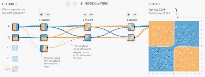
In contrast to other neural networks, Bayesian neural networks train the model weights as a distribution rather than searching for an optimal value. This makes them more robust and allows them to generalize better with less overfitting.
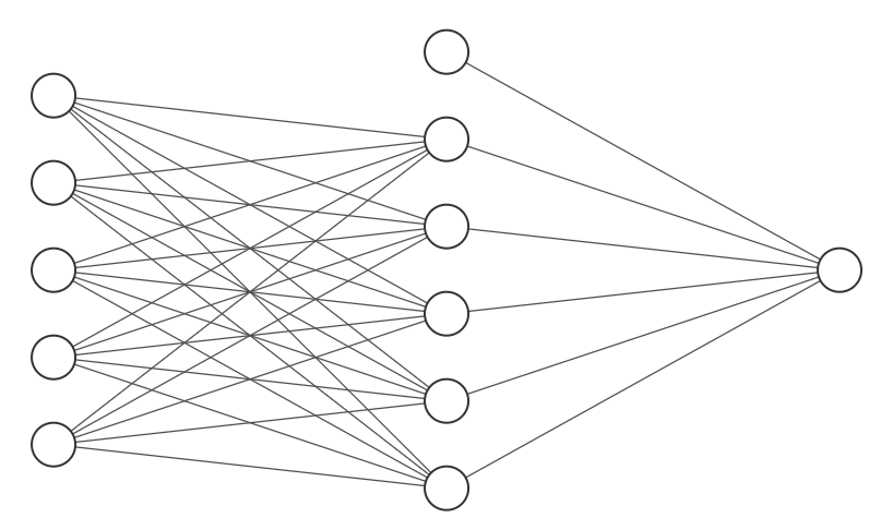
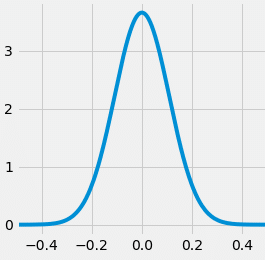
With standard neural networks, the weights between the different layers of the network take single values. In a Bayesian neural network the weights take on probability distributions. The process of finding these distributions is called marginalization.
One important factor for training these networks is having a large enough set of training data to produce accurate probability distributions.
Want to learn about methods for attempting to increase the size of your training data set? Check out my post about Data Augmentation!
Probabilistic Neural Networks
Probabilistic neural networks (PNNs) are a type of neural network that have outputs which are themselves a probability distribution.
The standard form of a bayesian neural network still outputs a single point estimate. If the network is run multiple times with the same inputs, this single point estimate will vary.
This is due to the nature of the network’s weights being probability distributions.
In contrast, a probabilistic neural network will output a distribution as the output. These two techniques can be combined to produce a probabilistic Bayesian neural network where both the network weights and the network outputs are distributions.
Bayesian (Deep) Learning a.k.a. Bayesian Inference
In statistics, Bayesian inference is a method of estimating the posterior probability of a hypothesis, after taking into account new evidence. The Bayesian approach to inference is based on the belief that all relevant information is represented in the data.
In other words, the data contains all the information needed to make a decision. This contrasts with frequentist inference, which relies on samples from a population.
Bayesian inference starts with a prior probability distribution (the belief before seeing any data), and then uses the data to update this distribution. The posterior probability is the updated belief after taking into account the new data.
One of the main benefits of Bayesian inference is that it can be used to model uncertainty, and this posterior distribution output is the mechanism by which a Bayesian probabilistic neural network will create the posterior distribution as output.
Bayesian deep learning is the practice of combining Bayesian inference with deep learning techniques.
Advantages and Disadvantages of Bayesian Neural Networks
There are many advantages to using Bayesian neural networks. Some of these include:
- They are more robust and able to generalize better than other neural networks.
- They can quantify the uncertainty in their predictive output.
- They can be used for many practical applications.
There are also some disadvantages to using Bayesian neural networks which we will now discuss.

As with any tool, these pros and cons must be weighed by the developer, engineer, or data scientist to determine whether the choice of neural network type is appropriate for the application. The Bayesian neural network is an important and effective tool to have in the belt, and should be considered when needed.
Some disadvantages include:
- They can be more complicated to train than other neural networks, and require knowledge of the fields of probability and statistics.
- They can be slower to converge than other neural networks and often require more data. Since the weights of the network are distributions instead of single values, more data is required to estimate the weights accurately.
In the next section, we’ll move on to making a Bayesian neural network using the popular libraries Keras and PyTorch.
If you’re more interested in the technical background for neural networks, don’t lose out on my article about content loss!
Or if you want to prevent overfitting, check out my post on if you should always use Dropout.
Making a Bayesian Neural Network in Python
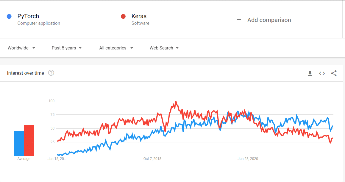
There are many great python libraries for modeling and using Bayesian neural networks. Two popular options include Keras and PyTorch. These libraries are well supported and have been in use for a long time.
Making a Bayesian Neural Network with Keras
Keras is a high-level neural networks library that provides a simplified interface for building neural networks. Keras is supported by Google and focuses on powerful results while using a simple and easier to use API. This allows for quick experimentation and prototyping.
We will follow along with Khalid Salama’s example in the Keras repository, which is licensed under the Apache License.
This tutorial uses chemical data about different wines to attempt to predict the wine quality. First, the libraries need to be installed. These include the Tensorflow probability library and the Tensorflow Datasets:
pip install tensorflow-probability
pip install tensorflow-datasets
Next, we need to import the needed python modules:
import numpy as np
import tensorflow as tf
from tensorflow import keras
from tensorflow.keras import layers
import tensorflow_datasets as tfds
import tensorflow_probability as tfp
To begin our script, we need to first import the training data, create the model inputs, and then create helper functions for assist with our experiment:
FEATURE_NAMES = [
    "fixed acidity",
    "volatile acidity",
    "citric acid",
    "residual sugar",
    "chlorides",
    "free sulfur dioxide",
    "total sulfur dioxide",
    "density",
    "pH",
    "sulphates",
    "alcohol",
]

hidden_units = [8, 8]
learning_rate = 0.001


def create_model_inputs():
    inputs = {}
    for feature_name in FEATURE_NAMES:
        inputs[feature_name] = layers.Input(
            name=feature_name, shape=(1,), dtype=tf.float32
        )
    return inputs

def get_train_and_test_splits(train_size, batch_size=1):
    # We prefetch with a buffer the same size as the dataset because th dataset
    # is very small and fits into memory.
    dataset = (
        tfds.load(name="wine_quality", as_supervised=True, split="train")
        .map(lambda x, y: (x, tf.cast(y, tf.float32)))
        .prefetch(buffer_size=dataset_size)
        .cache()
    )
    # We shuffle with a buffer the same size as the dataset.
    train_dataset = (
        dataset.take(train_size).shuffle(buffer_size=train_size).batch(batch_size)
    )
    test_dataset = dataset.skip(train_size).batch(batch_size)

    return train_dataset, test_dataset

def run_experiment(model, loss, train_dataset, test_dataset):

    model.compile(
        optimizer=keras.optimizers.RMSprop(learning_rate=learning_rate),
        loss=loss,
        metrics=[keras.metrics.RootMeanSquaredError()],
    )

    print("Start training the model...")
    model.fit(train_dataset, epochs=num_epochs, validation_data=test_dataset)
    print("Model training finished.")
    _, rmse = model.evaluate(train_dataset, verbose=0)
    print(f"Train RMSE: {round(rmse, 3)}")

    print("Evaluating model performance...")
    _, rmse = model.evaluate(test_dataset, verbose=0)
    print(f"Test RMSE: {round(rmse, 3)}")
The next step is to split the dataset into two groups. These groups are the training dataset which will be used to train the Bayesian neural network. The second set is the test dataset which will be used to validate the outputs. The split will be 85% of the data used in the training dataset, and 15% of the data in the test dataset:
dataset_size = 4898
batch_size = 256
num_epochs = 100
sample = 10
train_size = int(dataset_size * 0.85)

mse_loss = keras.losses.MeanSquaredError()

# Split the datasets into two groups
train_dataset, test_dataset = get_train_and_test_splits(train_size, batch_size)

# Sample some example targets from the test dataset
examples, targets = list(test_dataset.unbatch().shuffle(batch_size * 10).batch(sample))[
    0
]
Next, we must define the prior and posterior distributions for the Bayesian neural network weights:
def prior(kernel_size, bias_size, dtype=None):
    n = kernel_size + bias_size
    prior_model = keras.Sequential(
        [
            tfp.layers.DistributionLambda(
                lambda t: tfp.distributions.MultivariateNormalDiag(
                    loc=tf.zeros(n), scale_diag=tf.ones(n)
                )
            )
        ]
    )
    return prior_model

def posterior(kernel_size, bias_size, dtype=None):
    n = kernel_size + bias_size
    posterior_model = keras.Sequential(
        [
            tfp.layers.VariableLayer(
                tfp.layers.MultivariateNormalTriL.params_size(n), dtype=dtype
            ),
            tfp.layers.MultivariateNormalTriL(n),
        ]
    )
    return posterior_model
To create our Bayesian neural network, we need to define the helper function and a helper function which will compute predictions of the outputs:
def create_bnn_model(train_size):
    inputs = create_model_inputs()
    features = keras.layers.concatenate(list(inputs.values()))
    features = layers.BatchNormalization()(features)

    # Create hidden layers with weight uncertainty using the DenseVariational layer.
    for units in hidden_units:
        features = tfp.layers.DenseVariational(
            units=units,
            make_prior_fn=prior,
            make_posterior_fn=posterior,
            kl_weight=1 / train_size,
            activation="sigmoid",
        )(features)

    # The output is deterministic: a single point estimate.
    outputs = layers.Dense(units=1)(features)
    model = keras.Model(inputs=inputs, outputs=outputs)
    return model

def compute_predictions(model, iterations=100):
    predicted = []
    for _ in range(iterations):
        predicted.append(model(examples).numpy())
    predicted = np.concatenate(predicted, axis=1)

    prediction_mean = np.mean(predicted, axis=1).tolist()
    prediction_min = np.min(predicted, axis=1).tolist()
    prediction_max = np.max(predicted, axis=1).tolist()
    prediction_range = (np.max(predicted, axis=1) - np.min(predicted, axis=1)).tolist()

    for idx in range(sample):
        print(
            f"Predictions mean: {round(prediction_mean[idx], 2)}, "
            f"min: {round(prediction_min[idx], 2)}, "
            f"max: {round(prediction_max[idx], 2)}, "
            f"range: {round(prediction_range[idx], 2)} - "
            f"Actual: {targets[idx]}"
        )
Finally, we run the experiment and compute the predictions for the outputs:
num_epochs = 500
bnn_model_full = create_bnn_model(train_size)
run_experiment(bnn_model_full, mse_loss, train_dataset, test_dataset)

compute_predictions(bnn_model_full)
If all you needed was the Keras code, the next section will be the PyTorch example. Skip ahead to the Bayesian Neural Network FAQ!
Making a Bayesian Neural Network with PyTorch
PyTorch is a deep learning library that provides more flexibility in how the network is constructed, but can be more complicated to use. The library is supported by Facebook and provides the user with more comprehensive low level tools which require a broader knowledge.
With PyTorch, no out-of-the-box example exists, however a comprehensive library specific to Bayesian networks with PyTorch is maintained by Harry24k and is published under the MIT License. This tutorial will utilize this library and follow along with Harry24k’s example of the classification of iris data.
First, the library must be installed.
pip install torchbnn
Alternatively, you can use your favorite Python package or virtual environment manager like Anaconda or poetry.
Afterwards, the needed modules must be imported by our script:
import numpy as np
from sklearn import datasets

import torch
import torch.nn as nn
import torch.optim as optim

import torchbnn as bnn

import matplotlib.pyplot as plt
%matplotlib inline
At the beginning of our script, we have to load the iris data so that our Bayesian neural network can train with it.
iris = datasets.load_iris()

X = iris.data
Y = iris.target

x, y = torch.from_numpy(X).float(), torch.from_numpy(Y).long()
print(x.shape, y.shape)
Now that the data is loaded, the model, loss function, and optimizer must be defined. This example uses the Adam optimizer and two loss functions in the training process.
model = nn.Sequential(
    bnn.BayesLinear(prior_mu=0, prior_sigma=0.1, in_features=4, out_features=100),
    nn.ReLU(),
    bnn.BayesLinear(prior_mu=0, prior_sigma=0.1, in_features=100, out_features=3),
)

ce_loss = nn.CrossEntropyLoss()
kl_loss = bnn.BKLLoss(reduction='mean', last_layer_only=False)
kl_weight = 0.01

optimizer = optim.Adam(model.parameters(), lr=0.01)
With the model defined, the next step is to train the model with the iris data we loaded:
kl_weight = 0.1

for step in range(3000):
    pre = model(x)
    ce = ce_loss(pre, y)
    kl = kl_loss(model)
    cost = ce + kl_weight*kl

    optimizer.zero_grad()
    cost.backward()
    optimizer.step()

_, predicted = torch.max(pre.data, 1)
total = y.size(0)
correct = (predicted == y).sum()
print('- Accuracy: %f %%' % (100 * float(correct) / total))
print('- CE : %2.2f, KL : %2.2f' % (ce.item(), kl.item()))
Finally, the trained model must be tested and the results plotted.
def draw_plot(predicted) :
    fig = plt.figure(figsize = (16, 5))

    ax1 = fig.add_subplot(1, 2, 1)
    ax2 = fig.add_subplot(1, 2, 2)

    z1_plot = ax1.scatter(X[:, 0], X[:, 1], c = Y)
    z2_plot = ax2.scatter(X[:, 0], X[:, 1], c = predicted)

    plt.colorbar(z1_plot,ax=ax1)
    plt.colorbar(z2_plot,ax=ax2)

    ax1.set_title("REAL")
    ax2.set_title("PREDICT")

    plt.show()

pre = model(x)
_, predicted = torch.max(pre.data, 1)
draw_plot(predicted)
Bayesian Neural Network FAQ
Here are some frequently asked questions surrounding Bayesian neural networks:
The Naive Bayes algorithm is a probabilistic technique for classification which applies Bayes Theorem. It is based on the assumption that the features of each data point are independent of each other. This assumption is often violated in practice, but the algorithm still performs quite well in many cases. The Naive Bayes algorithm can be used with any type of data, including text, images, and vectors.
The Naive Bayes algorithm is so fast because it only requires calculating probabilities. This is in contrast to other classification algorithms, which might require computationally intensive training on the data. As a result Naive Bayes can be performed in real time.
Naive Bayes is a supervised technique because it applies Bayes’ theorem. Supervised learning is a type of machine learning where the computer is “trained” on a set of known data, and then used to make predictions on new data. The training data is used to teach the computer how to recognize patterns and make predictions. Unsupervised learning is a type of machine learning where the computer is “trained” on data that is not labeled. This means that the computer isn’t told what the data is supposed to be, it has to learn from scratch.
There are pros and cons of Naive Bayes classification.
The advantages are rooted in the fact that Naive Bayes is a simple calculation.
Pros: Easy implementation, Fast calculation which scales, Can be used with large data sets
Cons: Assumes random variables are independent, Limited applications can use this assumption
Some of the advantages to using Bayesian Neural Networks include:
-They are more robust and able to generalize better than other neural networks.
-They can quantify the uncertainty in their predictive output.
-They can be used for many practical applications.
Since Naive Bayes can be computed without neural networks it is not a neural network it is an algorithm. However, a neural network could be trained to implement the logic of the Naive Bayes algorithm.
The Naive Bayesian Classifier is a tool for performing classification tasks. A Bayesian Belief Network is a graphical model for representing the interactions between random variables using Bayesian Inference.
An example of Bayesian networks is any neural network which uses distributions for the weights in the network. They are used in cases where some information is known about the prior distributions of the random variables.
Bayesian neural networks allow the user to quantify the uncertainty in their predictive outputs.
Like all tools there are pros and cons of Bayesian Neural Networks.
Since these networks train an entire probability distribution rather than a single weight, they require more samples of training data than traditional neural networks.
There are many pros to using Bayesian neural networks. Some of these include:
-They are more robust and able to generalize better than other neural networks.
-They can quantify the uncertainty in their predictive output.
-They can be used for many practical applications.
There are also some cons to using Bayesian neural networks. Some of these include:
-They can be more complicated to train than other neural networks, and require knowledge of the fields of probability and statistics.
-They can be slower to converge than other neural networks and often require more data. Since the weights of the network are distributions instead of single values, more data is required to estimate the weights accurately.
For the most part, Bayesian neural networks are trained just like other networks, however they utilize a different technique called maximum a posteriori (MAP) estimation. This produces the probability distributions which make up the weights of the network.
A Bayesian Convolutional Neural Network uses the Bayesian network technique of expressing the network weights as probability distributions with a Convolutional Neural Network.
Bayesian deep learning is the practice of combining Bayesian inference with deep learning techniques.