
Visual Geometry Group (VGG) is a team of researchers at Oxford University that produced a common convolutional neural network (CNN) architecture. This now-famous CNN is also called VGG and became popular in 2014 after beating the famous 2012 AlexNet in a competition. If you want to know why VGG is so common and what makes it useful, you are in the right place.
VGG is a commonly used neural network because it performs well, it was produced by a trusted team from a prestigious university, it was trained for weeks on a massive set of training data, it generalizes well to different use cases, and it was released to the public for free.
It is one of the most prominent architectures used for testing image classification since 2014. Before we start to understand VGG better and cover its architecture, its uses, and its drawbacks, I want to highlight the major reasons it is so popular:
- Produced by a reputable and trusted team (VGG) at a prestigious university (Oxford)
- Trained for 2-3 weeks on 4 high-end GPUs which is not a training setup everyone can afford
- Advanced the state-of-the-art by using small 3×3 convolution filters and deeper networks
- Released to the public to help facilitate the advancement of the field
- Generalizes well to a variety of datasets in different areas so it is often used as a benchmarking tool
- Scored 1st and 2nd place in the 2014 ImageNet Large-Scale Visual Recognition Challenge (ILSVRC)
The competition of teams for the ILSVRC has motivated many advancements in the field of CNNs and computer vision generally. Let’s cover VGG in detail and why it is so useful.
What is VGG and What Uses Does It Have?
Table of Contents
VGG is a famous CNN architecture that first showed it was possible to do accurate image recognition with a deep network and small convolutional filters. It proved this to the world scoring highly in the ImageNet Challenge. The scoring for this challenge has two metrics. The “Top-1” metric examines how accurate the best guess is for classifying the image. The “Top-5” metric examines the best 5 guesses at classifying the image. If the correct category is in the best 5 guesses it considers the image correctly classified.
For Top-1, VGG was correct 76.3% of the time (23.7% error). For Top-5, VGG was correct 93.2% of the time (6.8% error). These impressive scores were far above the competition at the time and in an event where there are 1000 image categories to choose from. [1]
After AlexNet outperformed the competition in 2012 it spurred a huge interest in CNNs. Over the next few years, there was a flurry of investigations into the area and lots of attempts to improve on the technique. Some modifications that were investigated included examining the training data at different scales, orientations, and cropping. This is a technique called Data Augmentation and you can read all the details in my post about it!
In the 2013 competition, other networks also investigated using smaller convolutional filters. The VGG team led by Karen Simonyan and Andrew Zisserman (now of Google Deep Mind) recognized that combining this with a deeper network would increase the effective receptive field of the network and improve the accuracy.
The Receptive Field: Making VGG More Accurate
In CNNs, the receptive field refers to the area of the input image being examined by a node in the network. The term is borrowed from neuroscience and the visual field of neurons that process visual signals from the human eye.
For nodes early in the network, the receptive field might be only a few pixels. At deeper nodes, the receptive field might refer to an edge or shape within the image.
Still deeper nodes might recognize ‘eye’ or ‘wheel’ that are parts of the whole object. Finally, at the deepest nodes which recognize objects, the receptive field might be an entire person or car. [2]
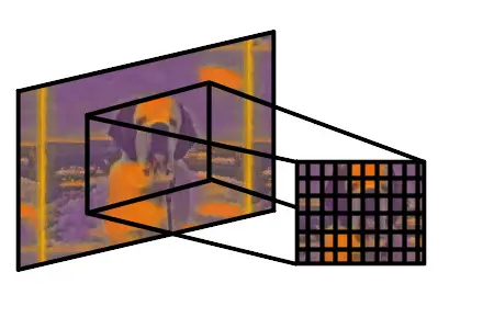
This image shows you the receptive field of one of the convolutional layers in the style transfer of Stella the St. Bernard puppy. After training the network, VGG can even be used to output images. Check out my post about whether CNNs and other neural networks can output images! Want to see the full results? Check out my post about the style transfers of Mark Rothko!
Some other style transfers you will enjoy:
- Express your creative side by checking out the Van Gogh Style Guide
- Peek at the masterpieces in the Picasso Style Guide
- Go on an abstract adventure with the Jackson Pollock Style Guide
- Get an impression of Monet’s masterpieces in the Monet Style Guide
- Journey through the symbolic depths with Frida Kahlo’s Style Guide
Earlier architectures tried to have larger receptive fields earlier in the network. VGG pioneered making the filter small (3×3) and the network deeper. By taking a stack of 3 convolutional layers with 3×3 filters, the stack has the same receptive field as a single 7×7 convolutional layer only with 45% fewer parameters to train. In addition, the activation is sharper than the single-layer design because the stack contains 3 activation functions. [1]
The Architecture of VGG Networks
As a general rule, the design of VGG is relatively traditional for a CNN. It follows the architecture principles of similar networks which were state-of-the-art at the time, and have been standardized since the earliest research into CNNs by LeCun in 1989. [3]
Usually, CNNs will have multiple convolutional layers (where these layers include the convolution and the activation function) followed by a pooling layer. In VGG, the activation is the ReLU function. This design, i.e. batches of layers, followed by pooling, is repeated as the network gets deeper. As a whole, the deeper layers will contain more filters than layers close to the input.
The larger number of filters allows the network to recognize a variety of complex shapes and objects. The early layers need to recognize shapes like lines and edges, while the deep layers might need to recognize cars or people. Since there is a larger number of complex object combinations, the deep layers contain the largest number of convolutional filters.
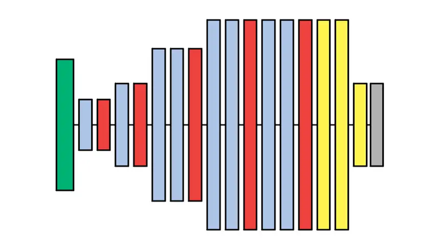
Finally, the deepest layers which are close to the output are linear fully connected layers. These layers convert the information passing through the network from a visual interpretation of image data to categories like ‘dog’, ‘cat’, or ‘person’. The final layer is a softmax function that converts the numerical value into a probability value for each category.
In the diagram, you can see the design of the VGG-A network. The different configurations will be discussed in the next section. The green layer is the input image, the blue layers are convolutional layers, the red layers are the max pooling layers, the yellow layers are the fully connected layers, and the gray layer is the softmax function before the output.
When common networks like VGG are used for other tasks a common approach is called Transfer Learning. A network like VGG has been trained on millions of images to recognize objects. The original competition had 1000 object categories, however, the user might only be interested in a different set of categories like ‘Hotdog’ and ‘Not Hotdog’. By freezing the weights of the convolutional layers, the final fully-connected layers can be trained for the new categories and VGG’s power can be reapplied to a novel task. [4]
Since the public release of our models, they have been actively used by the research community for a wide range of image recognition tasks, consistently outperforming more shallow representations.
Karen Simonyan and Andrew Zisserman [1]
The input image for VGG is a 224×224 image with 3 channels for Red, Green, and Blue however most commonly used neural network libraries like PyTorch, Keras, and Tensorflow have tools for transforming, scaling, cropping, and coloring images. These tools allow users to leverage existing trained networks like VGG with a wide variety of data sets.
Configurations of VGG
The original paper outlining the VGG architecture specified 6 different network configurations that were tested. Two configurations, D and E are now more commonly referred to as VGG16 and VGG19 respectively. The numbers refer to the number of weight layers that were trained in the network. I’ll cover each in detail.
The training process also included Dropout layers to help prevent overfitting. Want to learn more about Dropout? Check out my post tackling whether you should always use Dropout!
Configuration A and A-LRN
Configuration A was used to establish baseline performance and test Local Response Normalization (LRN). This technique had been used in previous CNN architectures which were popular at the time. The VGG paper showed that LRN does not contribute to a performance increase, yet requires more memory and more CPU processing.
In recent years LRN has fallen out of favor as a technique in favor of others like Batch Normalization. The VGG research was an influential paper that contributed to the decline of the technique as it was studied further.
| VGG-A Configuration |
|---|
| Input Image (224×244 pixels, 3 channels Red, Green, Blue) |
| Convolution Layer: 64 3×3 filters, stride 1, padding 1 (LRN Layer Optional) |
| Max Pooling Layer: 2×2 with stride 2 |
| Convolution Layer: 128 3×3 filters, stride 1, padding 1 |
| Max Pooling Layer: 2×2 with stride 2 |
| Convolution Layer: 256 3×3 filters, stride 1, padding 1 Convolution Layer: 256 3×3 filters, stride 1, padding 1 |
| Max Pooling Layer: 2×2 with stride 2 |
| Convolution Layer: 512 3×3 filters, stride 1, padding 1 Convolution Layer: 512 3×3 filters, stride 1, padding 1 |
| Max Pooling Layer: 2×2 with stride 2 |
| Convolution Layer: 512 3×3 filters, stride 1, padding 1 Convolution Layer: 512 3×3 filters, stride 1, padding 1 |
| Max Pooling Layer: 2×2 with stride 2 |
| Fully Connected Layer: 4096 nodes |
| Fully Connected Layer: 4096 nodes |
| Fully Connected Layer: 1000 nodes (one for each category) |
| Softmax |
Configuration B
This configuration added two extra convolutional layers over Configuration A. One of the motivations for training these smaller network configurations instead of immediately training the final configurations relates to initializing the weights.
During the optimization of the weights during backpropagation, there is the danger that the optimizer will not find a solution. There are sometimes thousands or millions of parameters to optimize for neural networks, and they all involve nonlinear functions so there is no guarantee that the optimizer will find the best solution.
One of the biggest factors in finding a good solution with nonlinear optimization is selecting where the initial conditions start. In this case, that’s the weights in the network that are being trained. The strategy for solving this issue was to first train the simple configurations like A, B, and C, and then later use the weights to initialize the more complex configurations like D and E.
| VGG-B Configuration |
|---|
| Input Image (224×244 pixels, 3 channels Red, Green, Blue) |
| Convolution Layer: 64 3×3 filters, stride 1, padding 1 Convolution Layer: 64 3×3 filters, stride 1, padding 1 |
| Max Pooling Layer: 2×2 with stride 2 |
| Convolution Layer: 128 3×3 filters, stride 1, padding 1 Convolution Layer: 128 3×3 filters, stride 1, padding 1 |
| Max Pooling Layer: 2×2 with stride 2 |
| Convolution Layer: 256 3×3 filters, stride 1, padding 1 Convolution Layer: 256 3×3 filters, stride 1, padding 1 |
| Max Pooling Layer: 2×2 with stride 2 |
| Convolution Layer: 512 3×3 filters, stride 1, padding 1 Convolution Layer: 512 3×3 filters, stride 1, padding 1 |
| Max Pooling Layer: 2×2 with stride 2 |
| Convolution Layer: 512 3×3 filters, stride 1, padding 1 Convolution Layer: 512 3×3 filters, stride 1, padding 1 |
| Max Pooling Layer: 2×2 with stride 2 |
| Fully Connected Layer: 4096 nodes |
| Fully Connected Layer: 4096 nodes |
| Fully Connected Layer: 1000 nodes (one for each category) |
| Softmax |
Configuration C
This configuration includes additional 1×1 Convolutional Layers. These layers do not affect the receptive field since they are 1×1 it is the same as the previous layer. However, the inclusion of the additional convolution and activation function increases the nonlinearity of the response. This configuration was used to compare and study the effect against the baseline of configuration B.
Despite being the same depth, Configuration C performed worse than Configuration D which is discussed in the next section. However, C did perform better than B.
| VGG-C Configuration |
|---|
| Input Image (224×244 pixels, 3 channels Red, Green, Blue) |
| Convolution Layer: 64 3×3 filters, stride 1, padding 1 Convolution Layer: 64 3×3 filters, stride 1, padding 1 |
| Max Pooling Layer: 2×2 with stride 2 |
| Convolution Layer: 128 3×3 filters, stride 1, padding 1 Convolution Layer: 128 3×3 filters, stride 1, padding 1 |
| Max Pooling Layer: 2×2 with stride 2 |
| Convolution Layer: 256 3×3 filters, stride 1, padding 1 Convolution Layer: 256 3×3 filters, stride 1, padding 1 Convolution Layer: 256 1×1 filters, stride 1 |
| Max Pooling Layer: 2×2 with stride 2 |
| Convolution Layer: 512 3×3 filters, stride 1, padding 1 Convolution Layer: 512 3×3 filters, stride 1, padding 1 Convolution Layer: 512 1×1 filters, stride 1 |
| Max Pooling Layer: 2×2 with stride 2 |
| Convolution Layer: 512 3×3 filters, stride 1, padding 1 Convolution Layer: 512 3×3 filters, stride 1, padding 1 Convolution Layer: 512 1×1 filters, stride 1 |
| Max Pooling Layer: 2×2 with stride 2 |
| Fully Connected Layer: 4096 nodes |
| Fully Connected Layer: 4096 nodes |
| Fully Connected Layer: 1000 nodes (one for each category) |
| Softmax |
Configuration D (a.k.a. VGG16)
In configuration D, there are 16 weighted layers present that need training. This is where it gets the name VGG16. A careful reader might notice the actual number of layers in VGG16 is 21, but the remaining 5 are Max Pooling layers that cannot be trained.
VGG16 is a network commonly used for benchmarking other networks and as an ‘out-of-the-box’ pre-trained network for image recognition tasks.
| VGG16 (VGG-D) Configuration |
|---|
| Input Image (224×244 pixels, 3 channels Red, Green, Blue) |
| Convolution Layer: 64 3×3 filters, stride 1, padding 1 Convolution Layer: 64 3×3 filters, stride 1, padding 1 |
| Max Pooling Layer: 2×2 with stride 2 |
| Convolution Layer: 128 3×3 filters, stride 1, padding 1 Convolution Layer: 128 3×3 filters, stride 1, padding 1 |
| Max Pooling Layer: 2×2 with stride 2 |
| Convolution Layer: 256 3×3 filters, stride 1, padding 1 Convolution Layer: 256 3×3 filters, stride 1, padding 1 Convolution Layer: 256 3×3 filters, stride 1, padding 1 |
| Max Pooling Layer: 2×2 with stride 2 |
| Convolution Layer: 512 3×3 filters, stride 1, padding 1 Convolution Layer: 512 3×3 filters, stride 1, padding 1 Convolution Layer: 512 3×3 filters, stride 1, padding 1 |
| Max Pooling Layer: 2×2 with stride 2 |
| Convolution Layer: 512 3×3 filters, stride 1, padding 1 Convolution Layer: 512 3×3 filters, stride 1, padding 1 Convolution Layer: 512 3×3 filters, stride 1, padding 1 |
| Max Pooling Layer: 2×2 with stride 2 |
| Fully Connected Layer: 4096 nodes |
| Fully Connected Layer: 4096 nodes |
| Fully Connected Layer: 1000 nodes (one for each category) |
| Softmax |
Configuration E (a.k.a. VGG19)
VGG19 is configuration E and is a more complex version of VGG16. It contains 3 additional convolutional layers in the image processing layers of the network. These layers are added fairly deeply into the architecture and add more variety for recognizing high-level shapes and objects.
During the experiments the performance improvement saturated at 19 layers, so the VGG researchers stopped adding layers with this configuration. However, this saturation could exist for only the ImageNet competition training set and does not rule out performance increases for deeper networks on other sets of training data. [1]
| VGG19 (VGG-E) Configuration |
|---|
| Input Image (224×244 pixels, 3 channels Red, Green, Blue) |
| Convolution Layer: 64 3×3 filters, stride 1, padding 1 Convolution Layer: 64 3×3 filters, stride 1, padding 1 |
| Max Pooling Layer: 2×2 with stride 2 |
| Convolution Layer: 128 3×3 filters, stride 1, padding 1 Convolution Layer: 128 3×3 filters, stride 1, padding 1 |
| Max Pooling Layer: 2×2 with stride 2 |
| Convolution Layer: 256 3×3 filters, stride 1, padding 1 Convolution Layer: 256 3×3 filters, stride 1, padding 1 Convolution Layer: 256 3×3 filters, stride 1, padding 1 Convolution Layer: 256 3×3 filters, stride 1, padding 1 |
| Max Pooling Layer: 2×2 with stride 2 |
| Convolution Layer: 512 3×3 filters, stride 1, padding 1 Convolution Layer: 512 3×3 filters, stride 1, padding 1 Convolution Layer: 512 3×3 filters, stride 1, padding 1 Convolution Layer: 512 3×3 filters, stride 1, padding 1 |
| Max Pooling Layer: 2×2 with stride 2 |
| Convolution Layer: 512 3×3 filters, stride 1, padding 1 Convolution Layer: 512 3×3 filters, stride 1, padding 1 Convolution Layer: 512 3×3 filters, stride 1, padding 1 Convolution Layer: 512 3×3 filters, stride 1, padding 1 |
| Max Pooling Layer: 2×2 with stride 2 |
| Fully Connected Layer: 4096 nodes (still ReLU) |
| Fully Connected Layer: 4096 nodes |
| Fully Connected Layer: 1000 nodes (one for each category) |
| Softmax |
Configurations Compared
At a high level, the different configurations have different numbers of trainable layers and a variety in the number of parameters that need to be trained. In general, the networks require training hundreds of millions of parameters.
As a result, if you are considering retraining these networks it requires a large number of training images. The base training set in the ImageNet competition contained 1.5 million images. In addition, the previously discussed Data Augmentation techniques were used to increase the number of available training images.
| VGG Configuration | Weight Layers | Number of Parameters |
|---|---|---|
| A and A-LRN | 11 Weight Layers | 133 Million |
| B | 13 Weight Layers | 133 Million |
| C | 16 Weight Layers | 134 Million |
| D (VGG16) | 16 Weight Layers | 138 Million |
| E (VGG19) | 19 Weight Layers | 144 Million |
This is a common reason that it is popular to reuse the weights of the already trained networks. In popular libraries like PyTorch, there is the torchvision package that contains many examples of common networks that have been trained. For VGG the torchvision package allows users to load weights for all of the different configurations.
Uses of VGG
The VGG networks can be used for any task that image recognition is used for. This includes (but not exclusively) the following applications:
- Object detection and recognition
- Localization (i.e. locating an object)
- Character recognition and text processing
- Style transfers
- Generating images (using the network in reverse like Google’s Deep Dream)
- Artificially generating missing information from images or increasing the resolution
- Image editing tools
- Face recognition
- Self Driving Cars
Want to learn more about how CNNs like the VGG network are used in Style Transfer artwork? Check out my post discussing content and style loss!
Benefits and Drawbacks of VGG
Some of the benefits of the VGG network include:
- Easy to understand conceptually – standard architecture for CNNs
- Well researched and widely used. Great for understanding CNN concepts.
- Available in most popular machine learning libraries
- Good performance at image classification and generalizes well to related tasks
- Trained for weeks on millions of images
Some of the drawbacks of the VGG network include:
- Research has continued since 2014 and there are often better-performing CNN architectures available
- With over 100 million trained weights, the model size is large. ~500MB on disk.
- Training for a different task (transfer learning) can be difficult due to the deep network and vanishing gradient problem
I always found the architecture of VGG to be educational for its simplicity in design. Many more recent network designs base their decisions off standard practice that was influenced by VGG.
Frequently Asked Questions
Resnet is a more recent CNN architecture that uses less memory than VGG, allows for deeper networks with more layers, and performs inference faster than VGG. The needs of the user vary from application to application so the choice of network design should depend on the required accuracy and performance requirements of the task at hand. For some training sets, deeper networks can have higher error rates and generalize worse than simpler networks.
The only difference between VGG16 and VGG19 is that VGG19 has three extra convolutional layers. The other features like pooling layers, fully connected layers, and classification channels are the same for both networks.
Final Thoughts on VGG
Now that you know why VGG is such a commonly used network, you can use it for your own in-depth object detection, image recognition, and image classification tasks. The VGG network generalizes well to many training sets in applied fields such as medicine, robotics, automotive, etc. Due to its long history and wide availability, it is one of the most commonly referenced architectures for image classification.
Want to learn more about style transfers and how they are used in digital art? Check out my post completely covering the topic!
Another common type of network is a Bayesian Neural Network. Want to learn how this network type deals with uncertainty? Check out my post about Bayesian Neural Networks in Python!
Get Notified When We Publish Similar Articles
References
- Simonyan, Karen, and Andrew Zisserman. “Very deep convolutional networks for large-scale image recognition.” arXiv preprint arXiv:1409.1556 (2014).
- Araujo, et al., “Computing Receptive Fields of Convolutional Neural Networks”, Distill, 2019.
- LeCun, Yann, et al. “Backpropagation applied to handwritten zip code recognition.” Neural computation 1.4 (1989): 541-551.
- Tammina, Srikanth. “Transfer learning using vgg-16 with deep convolutional neural network for classifying images.” International Journal of Scientific and Research Publications (IJSRP) 9.10 (2019): 143-150.