Neural style transfer is the ability to separate the style and content of images using a Convolutional Neural Network (CNN). In neural style transfer, you have endless possibilities of applying an entirely different style to an existing image. The style can be anything you like, from cubism, surrealism, impressionism, or something of your own creation. It uses several different loss functions including content loss.
The content loss in neural style transfer is the distance (L2 Norm) between the content features of a base image and the content features of a generated image with a new style. The content of the generated image has to be similar to the base. This is ensured by minimizing the content loss score.
There are a lot of underlying motivations for using content loss in neural style transfer. To understand it better, one must know how to calculate it. So, if you are interested in all this information, read further!
Introduction to Content Loss in Neural Style Transfer
Table of Contents
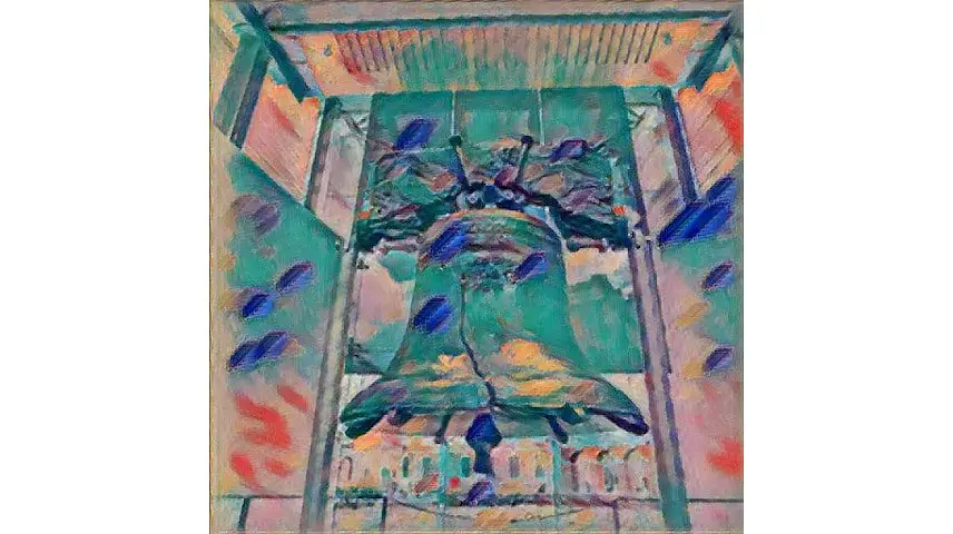
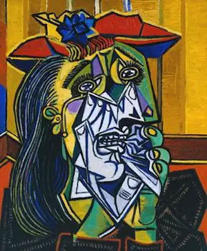
Neural style transfer is a way of generating an image using the content of a picture but with a different style generally taken from an artistic image or painting. A great example would be a picture of a swan with the style of a cubist like Picasso.
Both the images are blended to get a new, unique and creative image. In neural style transfer, you find three different types of loss namely:
- Content Loss
- Style Loss
- Total Variation Loss
To understand neural style transfer better, you need to learn about these losses. Loss calculation is a large part of this algorithm.
If you like Picasso’s style, Peek at Picasso’s paintings by checking out the Picasso Style Guide.


Content Loss
In the content loss, the features of the generated image are compared to the content image. It is to make sure that the generated image has the same content while the algorithm changes the style. This way, the authenticity of the content image isn’t lost and from the style image, the style elements get added.
First, two copies of the same pre-trained image classification CNNs are used as loss networks. These networks will be fed a reference image (content) and a test image (generated) respectively. The outputs from these two classifiers are used as inputs to the loss function.
In plain English, the calculation is a distance (Euclidean) between two contents output from the loss CNNs; one content from the generated image and the other from the base image. [2]
Calculation of Content Loss Function
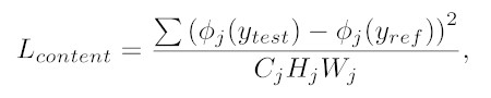
To calculate the content loss function, you have to calculate two things first. The content features of both the generated image and the content image using the pre-trained loss networks. Next, the Mean Squared Error (a.k.a. the L2 Norm) is calculated.
To perform this calculation, we follow the name. First, calculate the error using element-wise subtraction. Subtract the generated image features from the content image features.
Next, square these errors element-wise to get the squared errors. Add all the values and divide by the number of features to calculate the average, and you will have the Mean Squared Error.
Content Loss Using Pytorch
Using Pytorch, the content loss calculation is as follows:
# Move the image to the GPU (or CPU using regular FloatTensor)
# and generate the transferred image y_hat with new style
x = Variable(x).type(torch.cuda.FloatTensor).to(device)
y_hat = image_transformer(x).to(device)

# Calculate features using VGG image classifiers
ref_features = vgg(x)
test_features = vgg(y_hat)

# get the MSE Loss function
loss_mse = torch.nn.MSELoss()

# What layer within the CNN to calculate the content loss. Low layers (0, 1...) have low
# level features like lines. High layers have object classifications like 'eye' or 'car'
content_feature = 1

# calculate the content loss
content_loss = content_weight * loss_mse(ref_features[content_feature], test_features[content_feature])
In this example code, vgg and image_transformer are both torch.nn.Module objects which implement a neural network within the Pytorch library. The vgg objects are the loss networks, and image_transformer is the style transfer network being trained.
These VGG networks are from the torchvision package which implements famous and frequently used neural networks. VGG is a CNN for image classification that was trained on millions of images. Want to learn more about why VGG is so commonly used? Check out my post covering this influential network!
The content_weight is a parameter chosen by the user to subjectively determine how much to weigh the content vs the style. It changes for each style being trained.
This explanation is a simple way to describe the formula of content loss which can look intimidating at first. Hopefully, I have summed it up for you – in style!
Reason for Content Loss
You might be wondering why content loss is so important in neural style transfer. Well, it’s simple!
The content loss ensures that the resulting image has similar activations as the base image in the higher layers. Content loss deals with the activations of higher layers whereas lower layers are dealt with by style and other losses. Therefore, to achieve a perfect and efficient image, content loss is important.
How to Implement the Loss in Neural Style Transfer?
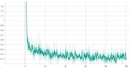
Implementing loss in neural style transfer takes a particular approach. When you add a training image to the neural network, the autograd system of the library being used (in this post, Pytorch) computes all the gradients. So, all the losses are computed for every single desired layer. The weights will be updated so that the total loss is minimized.
By using the above formulas for calculating the content loss value, you can take the content loss of one or more layers. Take them as an additive module for the neural transfer.
Next, the other losses need to be calculated so that we can calculate the total loss by summing them.
Content Loss vs Style Loss
Another important loss is the style loss which is represented by the gram matrix. It is important to learn the difference between the two losses to understand them better. You can’t implement neural style transfer without these two.
So, what is style loss? In simple words, style loss is the measure of how different the lower-level features of the generated image are from the base image. For example, features like color and texture.
Style loss is obtained from all the layers whereas content loss is obtained from higher layers. It goes into the deepest of layers to make sure that there is a visible difference between the style image and the generated image. After all, we don’t want the original image to lose its value and real meaning.
The concept of content loss is far easier than style loss. For content loss, you can use a simple mathematical formula to find out its value. The implementation of content loss is also less complicated. Let’s see how the style loss is calculated!
Style Loss Calculation
The style loss is meant to penalize the output image when the style is deviating from the supplied style image. Now, for content loss, you can simply add up and divide for the Mean Squared Error value. For style loss, there is another step.
First, a loss network is used like with the content loss. Both the test (generated) image features and style image features are fed to the loss networks. This produces their activations.
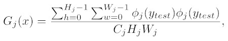
Next, these outputs are averaged over every value in the feature map to calculate the Gram matrix. This matrix is a measurement of the style at each layer. The matrix measures covariance and therefore it captures information about regions of the image which tend to activate together. The benefit of using a gram matrix is that it enables different features to co-exist in different parts of the images.
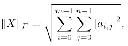
After the gram matrix, the style loss is a squared distance (i.e. error) between the gram matrix of the generated image and the gram matrix of the style image. In this case, the distance is called the Frobenius norm because it is measuring the distance between two matrices. It is an extension of the Euclidean norm for matrices.
These additional steps make the style loss more complex and its calculation and implementation more effort. There are also approximation methods for Gram Matrices to speed up their calculation. [1]
Style loss is obtained from all the layers whereas content loss is obtained from higher layers. It goes into the deepest of layers to make sure that there is a visible difference between the style image and the generated image. After all, we don’t want the original image to lose its value and real meaning.
Calculating the Style Loss in Pytorch. This alternate implementation uses MSE:
def gram(x):
    # get the batch size, channels, height, and width of the image
    (bs, ch, h, w) = x.size()
    f = x.view(bs, ch, w * h)
    G = f.bmm(f.transpose(1, 2)) / (ch * h * w)
    return G

# Move the image to the GPU (or CPU using regular FloatTensor)
# and generate the transferred image y_hat with new style
x = Variable(x).type(torch.cuda.FloatTensor).to(device)
y_hat = image_transformer(x).to(device)

# Calculate features using VGG image classifiers
test_features = vgg(y_hat)
style_features = vgg(style)

# Get the gram matrices
style_gram = [gram(fmap) for fmap in style_features]
test_gram = [gram(fmap) for fmap in test_features]

# Calculate the style loss (mse demo)
style_loss = 0.0
for j in range(4):
    style_loss += loss_mse(test_gram[j], style_gram[j][:img_num])

style_loss = style_weight * style_loss
Gram Matrix
To understand style loss and the difference between style loss and content loss, it is important to learn about gram matrices.
Gram matrix measures how much correlation there is between all the style feature maps. It calculates the features of every layer of a style.
The Gram matrix is used to determine the calculation for all the particular styles for both the generated image and the style image.
Total Loss
After calculating both style loss and content loss, you need to find out the total loss.
Total loss is simply the sum of the content loss and style loss. By finding out the total loss, you can understand how the optimizer is finding an image that has the style of one image and the content of another.
total_loss = style_loss + content_loss
By controlling the total loss with the user-defined content weight and style weight, you can either have a more artistic image or an image with more features but less style or art.
Want to check out some style transfers that were made using these loss concepts?
- Express yourself with the Van Gogh Style Guide.
- Go on an abstract adventure with the Jackson Pollock Style Guide
- Get an impression of Monet’s masterpieces in the Monet Style Guide
- Take a Rothko Retrospective with the Mark Rothko Style Guide
- Journey through the symbolic depths with Frida Kahlo’s Style Guide
- Discover Dali’s surreal style with the Salvador Dali Style Guide
Want to learn more about how style transfers and neural networks work?
- Want to know about Dropout and whether you should use it in your own networks? Check out my post on if you should always use Dropout.
- If you want to improve the quality of the networks you train, learn more about Data Augmentation!
Frequently Asked Questions
Final Thoughts
Now that you know how the content and the style loss work in neural style transfer, you can easily edit your photos using different styles and create your own artwork. Getting an artistic photo can become easier once you learn all the aspects of neural style transfer which also includes content loss.
Style loss and content loss are the two important loss functions in neural style transfer. Without understanding these two, their differences, and calculation, you can’t comprehend neural style transfer. So, implement this creative system in your photos to get the best results!
For more information on other types of neural networks, check out our tutorial on Bayesian Neural Networks and how to create them using two different popular python libraries.
Want to see an overview and the history of style transfers? Check out my post on Style Transfers, Neural Networks, and Digital Art! If you want to know other ways neural networks output images, check out my post on it!
Check out some other posts in the Style Transfer Category to learn more on this stellar topic.
Get Notified When We Publish Similar Articles
References
- Drineas, Petros, Michael W. Mahoney, and Nello Cristianini. “On the Nyström Method for Approximating a Gram Matrix for Improved Kernel-Based Learning.” journal of machine learning research 6.12 (2005). https://www.jmlr.org/papers/volume6/drineas05a/drineas05a.pdf
- Johnson, Justin, Alexandre Alahi, and Li Fei-Fei. “Perceptual losses for real-time style transfer and super-resolution.” European conference on computer vision. Springer, Cham, 2016, https://link.springer.com/chapter/10.1007/978-3-319-46475-6_43